Modulo Scheduling In HLS (Loop Pipeline Synthesize)
Modulo Scheduling In HLS (Loop Pipeline synthesis)
Instruction Scheduling Introduction
Instruction Scheduling can be broken into three categories: Local Scheduling, Global Scheduling, and Cyclic Scheduling:
- Local Scheduling handles single basic blocks which are regions of straight line code that have a single entry and exit (List scheduling).
- Global Scheduling can handle multiple basic blocks with acyclic control flow (Trace Scheduling, Superblock Scheduling, Hyperblock Scheduling).
- Cyclic Scheduling handles single or multiple basic blocks with cyclic control flow. (Modulo Scheduling)
There exist many Global Scheduling algorithms that can also be used in cyclic scheduling
- Trace Scheduling It identifies frequently executed traces in the program and treats the path as an extended basic block which is scheduled using a list scheduling approach.
- Superblock Scheduling Superblocks are a subset of traces which have a single entry and multiple exit attributes (therefore they are traces without side exits). List scheduling is typically used to schedule the superblock.
- Hyperblock Scheduling Excessive control flow can complicate scheduling, so this approach uses a technique called If-Conversion to remove conditional branches.
General Steps Of Modulo Scheduling
Modulo Scheduling is traditionally restricted to single basic block loops without control flow, which can limit the number of candidate loops. Global Software Pipelining techniques have emerged to exploit some of the opportunities for ILP in multiple basic block loops that frequently occur in computation intensive applications.
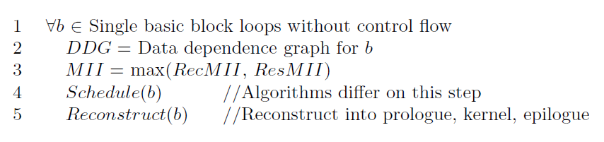
Using the DDG, the Minimum Initiation Interval (MII), which is the minimum amount of time between the start of successive iterations of a loop, is computed. Modulo Scheduling algorithms aim to create a schedule with an Initiation Interval (II) equal to MII, which is the smallest II possible and results in the most optimal schedule. The lower the II, the greater the parallelism.
Using the MII value as their initial II value, the algorithms attempt to schedule each instruction in the loop using some set of heuristics. If an optimal schedule can not be obtained, II is increased, and the algorithm attempts to compute the schedule again. This process is repeated until a schedule is obtained or the algorithm gives up. From this schedule, the loop is then reconstructed into a prologue, a kernel, and an epilogue. The prologue begins the first n iterations. After n ∗ II cycles, a steady state is achieved and a new iteration is initiated every II cycles. The epilogue finishes the last n iterations. Loops with long execution times will spend the majority of their time in the kernel.
Main Steps
Data Dependency Graph construction
There are three types of dependencies in the DDG:
- True Dependence: If the first instruction writes to a value, and a second instruction reads the same value, there is a true dependence from the first instruction to the second.
- Anti Dependence: If the first instruction reads a value, and a second instruction writes a value, then there is an anti dependence from the first instruction to the second.
- Output Dependence: If two instructions both write to the same value, then there is an output dependence between them.
Each dependence has a distance associated with it, called the iteration difference. If the distance is zero, this means the dependence is a loop-independent dependence, in other words a dependence within one iteration. If the distance is greater than zero, there is a dependence across iterations, a loop-carried dependence. The value of the distance for loop-carried dependences is one (a conservative guess), unless further analysis can prove the actual number of iterations between the instructions. The distance can also be calculated using SCEV and AA analysis, for details info, please refer to Chapter4.2 of this artical
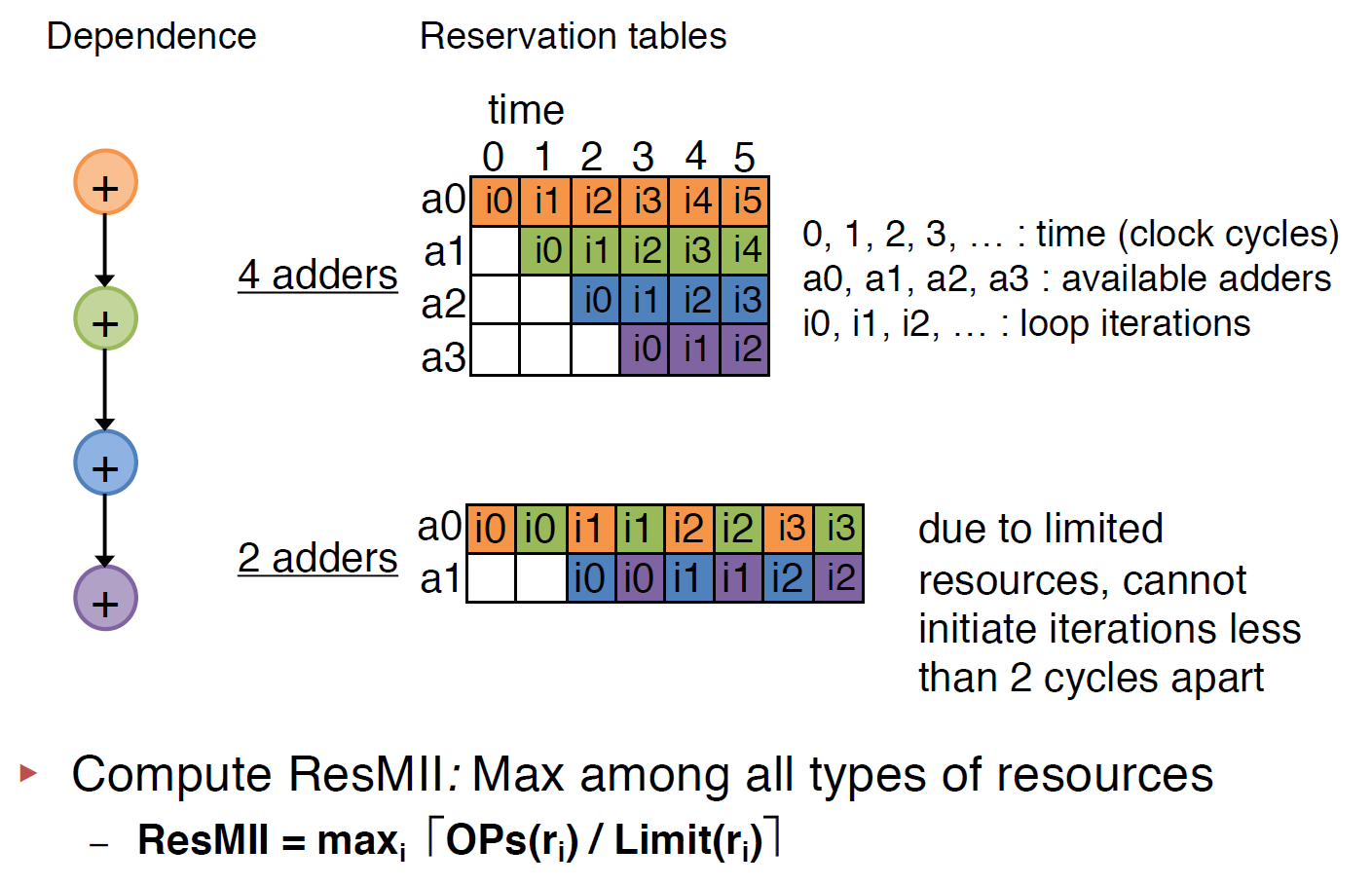
Calculating the Minimum Initiation Interval
Resource II (Heuritic, exact method is NP-hard)
Recurrence II
Recurrences may be found in the the DDG if instructions have dependences across iterations of the loop. Memory operations (load/store) are most likely the cause of a recurrence in the DDG. Recurrences are also known as circuits or cycles.
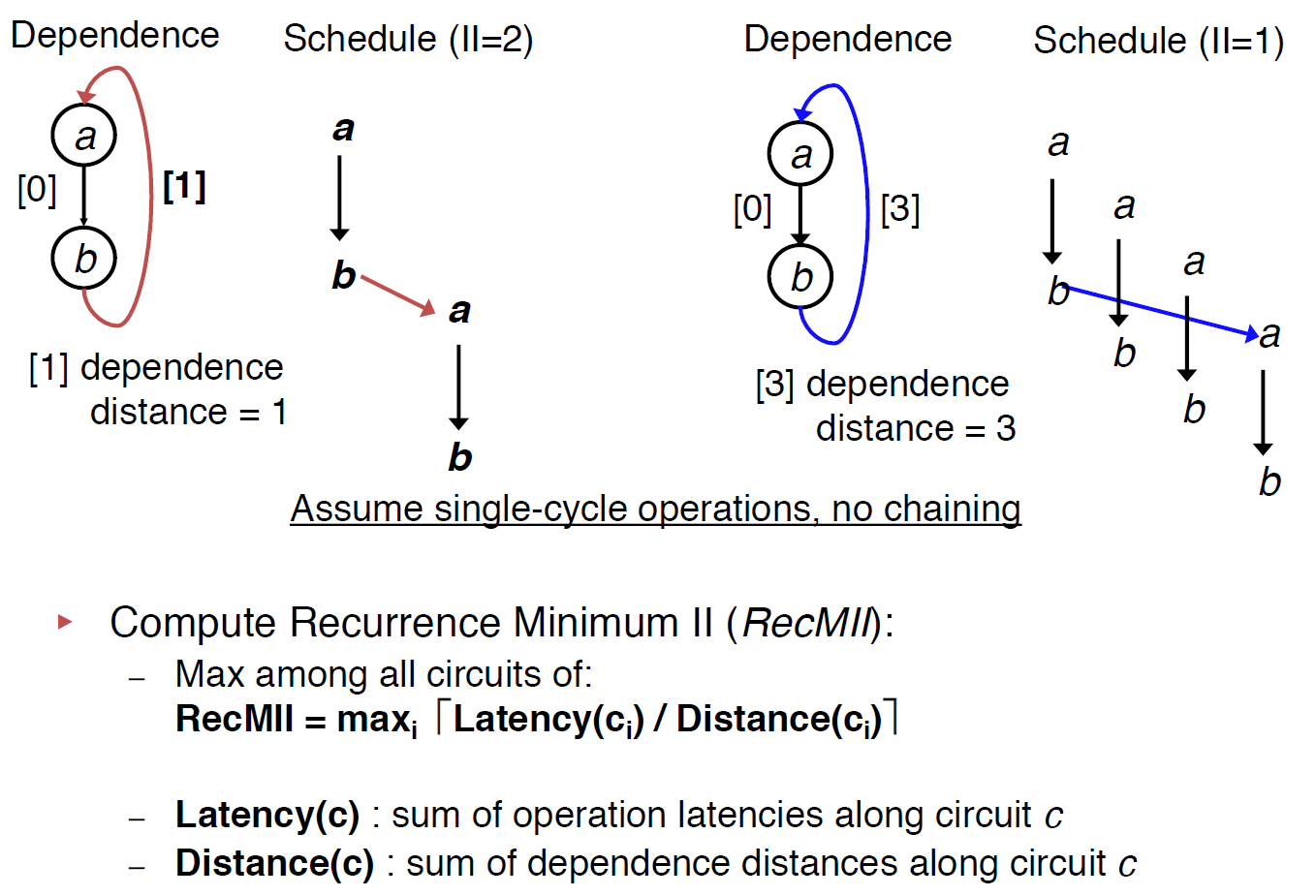
In order to compute the Recurrence Minimum Initiation Interval (RecMII), all recurrences in the DDG must be found. the algorithm proposed by Donald Johnson is used to find all elementary circuits in the DDG. If no vertex except the first and last appear twice, then a circuit is termed elementary (I found an excellent video about implementation and explanation of this algorithm).
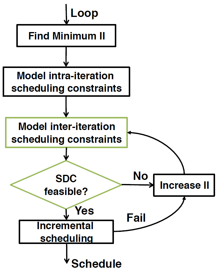
SDC-based Scheduling
Modeling Loop-Carried Dependence with SDC
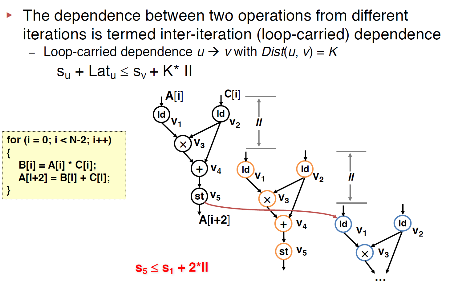
This was just end(u) - start(v) <= II * dis(u,v) where end(u) is the cycle time when the output of operation u is available, and start(v) is the starting cycle of operation v, for the above example, u is v5 and v is v1 . Note that Lat(u) is counted by cycles not the real latency, for instance, if the add takes 2ns to finish and the cycle time is 5ns then, the Lat(add) = 0, where, if the add takes 6ns, the Lat(add) = 1.
Inter-Iteration Cycle Time Constraint with SDC
Loop pipelining exposes possibili- ties of chaining operations across iterations; namely, the result produced by an operation can be directly consumed in the same clock cycle by another operation that belongs to a later iteration. If such a path exists and involves one or mul- tiple inter-iteration dependences (i.e., back edges), we need to construct the following constraint to ensure that a register is inserted on this path to prevent the unfavorable cross- iteration chaining from causing a frequency violation.
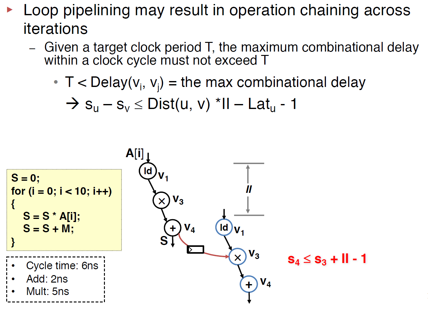
The above constraint can also be rewrote to s(v) + II*Dis(u,v) > s(u) + Lat(u), note that, here we use > instead of >= since the -1 is dropped.
Resource Constraint with Modulo Reservation Table (MRT)
Given resource constraints, we keep track of available resources using a table, where each row tracks a resource and each column is an available time slot. When we schedule an operation at time t, we reserve a single time slot in column t mod II of the table and in the appropriate resource row. Consequently the table is called the modulo reservation table (MRT) and has II time slot columns.